Reference mass balance data#
Traditional in-situ MB data#
In-situ mass balance data are used by OGGM to calibrate and validate the first generation mass balance model. We rely on mass balance observations provided by the World Glacier Monitoring Service (WGMS). The Fluctuations of Glaciers (FoG) database contains annual mass balance values for several hundreds of glaciers worldwide. We exclude water-terminating glaciers and the time series with less than five years of data. Since 2017, the WGMS provides a lookup table linking the RGI and the WGMS databases. We updated this list for version 6 of the RGI, leaving us with 268 mass balance time series. These are not equally reparted over the globe:
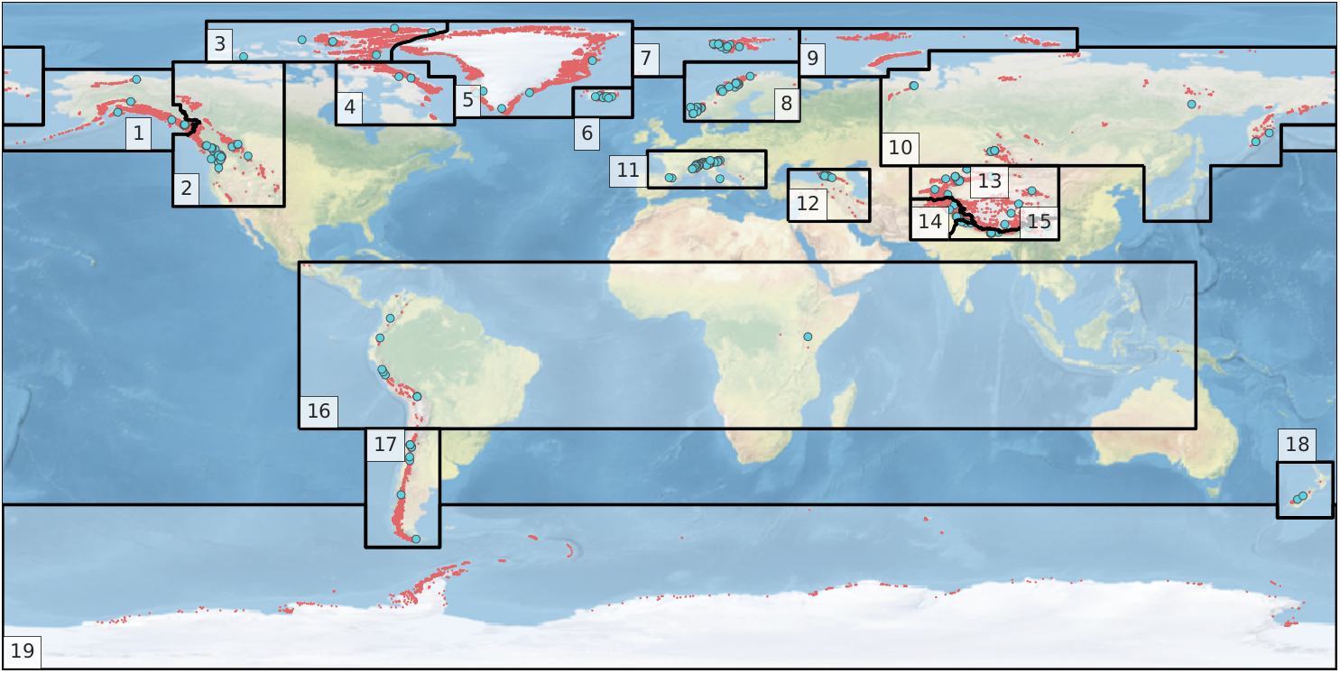
Map of the RGI regions; the red dots indicate the glacier locations and the blue circles the location of the 254 reference WGMS glaciers used by the OGGM calibration. From our GMD paper.#
These data are shipped automatically with OGGM. All reference glaciers have access to the timeseries through the glacier directory:
In [1]: gdir = workflow.init_glacier_directories('RGI60-11.00897',
...: from_prepro_level=5,
...: prepro_base_url=DEFAULT_BASE_URL,
...: prepro_border=80)[0]
...:
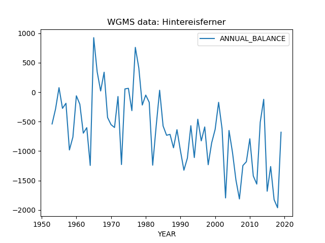
In [2]: mb = gdir.get_ref_mb_data()
In [3]: mb[['ANNUAL_BALANCE']].plot(title='WGMS data: Hintereisferner');
Geodetic MB data#
OGGM ships with a geodetic mass balance table containing MB information for all of the world’s glaciers as obtained from Hugonnet et al., 2021.
The original, raw data have been modified in three ways (code):
the glaciers in RGI region 12 (Caucasus) had to be manually linked to the product by Hugonnet because of large errors in the RGI outlines. The resulting product used by OGGM in region 12 has large uncertainties.
outliers have been filtered as following: all glaciers with an error estimate larger than 3 \(\Sigma\) at the RGI region level are filtered out
all missing data (including outliers) are attributed with the regional average.
You can access the table with:
In [4]: from oggm import utils

In [5]: mbdf = utils.get_geodetic_mb_dataframe()

In [6]: mbdf.head()
Out[6]:
                               period      area  ...  reg  is_cor
rgiid                                            ...
RGI60-01.00001  2000-01-01_2010-01-01  360000.0  ...    1   False
RGI60-01.00001  2000-01-01_2020-01-01  360000.0  ...    1   False
RGI60-01.00001  2010-01-01_2020-01-01  360000.0  ...    1   False
RGI60-01.00002  2000-01-01_2010-01-01  558000.0  ...    1   False
RGI60-01.00002  2000-01-01_2020-01-01  558000.0  ...    1   False

[5 rows x 6 columns]
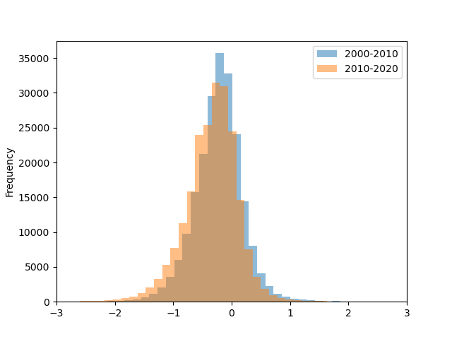
The data contains the climatic mass balance (in units meters water-equivalent per year) for three reference periods (2000-2010, 2010-2020, 2000-2020):
In [7]: mbdf['dmdtda'].loc[mbdf.period=='2000-01-01_2010-01-01'].plot.hist(bins=100, alpha=0.5, label='2000-2010');

In [8]: mbdf['dmdtda'].loc[mbdf.period=='2010-01-01_2020-01-01'].plot.hist(bins=100, alpha=0.5, label='2010-2020');

In [9]: plt.xlabel(''); plt.xlim(-3, 3); plt.legend();
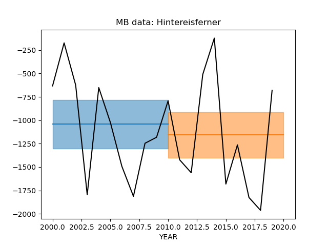
Just for fun, here is a comparison of both products at Hintereisferner:
In [10]: sel = mbdf.loc[gdir.rgi_id].set_index('period') * 1000

In [11]: _mb, _err = sel.loc['2000-01-01_2010-01-01'][['dmdtda', 'err_dmdtda']]

In [12]: plt.fill_between([2000, 2010], [_mb-_err, _mb-_err], [_mb+_err, _mb+_err], alpha=0.5, color='C0');

In [13]: plt.plot([2000, 2010], [_mb, _mb], color='C0');

In [14]: _mb, _err = sel.loc['2010-01-01_2020-01-01'][['dmdtda', 'err_dmdtda']]

In [15]: plt.fill_between([2010, 2020], [_mb-_err, _mb-_err], [_mb+_err, _mb+_err], alpha=0.5, color='C1');

In [16]: plt.plot([2010, 2020], [_mb, _mb], color='C1');

In [17]: mb[['ANNUAL_BALANCE']].loc[2000:].plot(ax=plt.gca(), title='MB data: Hintereisferner', c='k', legend=False);