Ice dynamics
The glaciers in OGGM are represented by a depth integrated flowline model. The equations for the isothermal shallow ice are solved along the glacier centerline, computed to represent best the flow of ice along the glacier (see for example antarcticglaciers.org for a general introduction about the various type of glacier models).
Here we present the basic physics and numerics of the two models implemented currently in OGGM, the FluxBasedModel (homegrown model with a rather simple numerical solver) and the MUSCLSuperBeeModel (mass-conserving numerical scheme, see [Jarosch_etal_2013]).
Basics
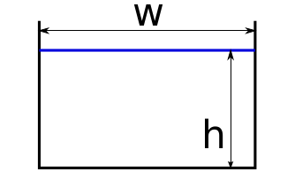
Let \(S\) be the area of a cross-section perpendicular to the flowline. It has a width \(w\) and a thickness \(h\) and, in this example, a parabolic bed shape.
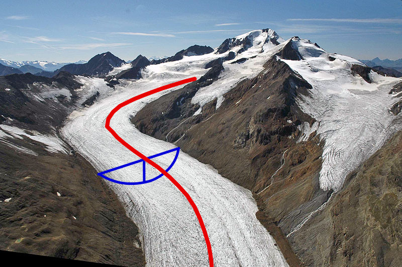
Example of a cross-section along the glacier flowline. Background image from http://www.swisseduc.ch/glaciers/alps/hintereisferner/index-de.html
Volume conservation for this discrete element implies:
where \(\dot{m}\) is the mass-balance, \(q = u S\) the flux of ice, and \(u\) the depth-integrated ice velocity ([Cuffey_Paterson_2010], p 310). This velocity can be computed from Glen’s flow law as a function of the basal shear stress \(\tau\):
The second term is to account for basal sliding, see e.g. [Oerlemans_1997] or [Golledge_Levy_2011]. It introduces an additional free parameter \(f_s\) and will therefore be ignored in a first approach. The deformation parameter \(f_d\) is better constrained and relates to Glen’s temperature‐dependent creep parameter \(A\):
The basal shear stress \(\tau\) depends e.g. on the geometry of the bed [Cuffey_Paterson_2010]. Currently it is assumed to be equal to the driving stress \(\tau_d\):
where \(\alpha\) is the slope of the flowline and \(\rho\) the density of ice. Both the FluxBasedModel and the MUSCLSuperBeeModel solve for these equations, but with different numerical schemes.
Bed thickness inversion
To compute the initial ice thikness \(h_0\), OGGM follows a methodology largely inspired from [Farinotti_etal_2009] but using a different apparent mass-balance (see also: Mass-balance) and another calibration algorithm.
The principle is simple. Let’s assume for now that we know the ice velocity \(u\) along the flowline of our present-time glacier. Then the above equations can be used to compute the section area \(S\) out of \(u\) and the other ice-flow parameters. Since we know the present-time width \(w\) with accuracy, \(h_0\) can be obtained by assuming a certain geometrical shape for the bed.
In OGGM, a number of climate and glacier related parameters are fixed prior to the inversion, leaving only one free parameter for the calibration of the bed inversion procedure: the inversion factor \(f_{inv}\). It is defined such as:
With \(A_0\) the standard creep parameter (2.4e-24). Currently, \(f_{inv}\) is calibrated to minimize the volume RMSD of all glaciers with a volume estimation in the GlaThiDa database. It is therefore neither glacier nor temperature dependent and does not account for uncertainties in GlaThiDa’s glacier-wide thickness estimations, two approximations which should be better handled in the future.
Flux based model
Most flowline models treat the volume conservation equation as a diffusion problem, taking advantage of the robust numerical solutions available for this type of equations. The problem with this approach is that it develops the \(\partial S / \partial t\) term to solve for ice thikness \(h\) directly, thus implying different diffusion equations for different bed geometries (e.g. [Oerlemans_1997] with a trapezoidal bed).
The OGGM flux based model solves for the \(\nabla \cdot q\) term on a staggered grid (hence the name). It has the advantage that the model numerics are the same for any bed shape, but it makes one important simplification: the stress \(\tau = \alpha \rho g h\) is always the same, regardless of the bed shape. This doesn’t mean that the shape has no influence on the glacier evolution, as explained below.
Glacier bed shapes
OGGM implements a number of possible bed-shapes. Currently the shape has no direct influence on ice dynamics, but it does influence how the width of the glacier changes with ice thickness and thus will influence the mass-balance \(w \, \dot{m}\). It appears that the flowline model is quite sensitive to the bed shape.
TrapezoidalFlowline
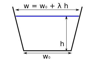
Trapezoidal shape with two degrees of freedom. The width change with thickness depends on \(\lambda\). [Golledge_Levy_2011] uses \(\lambda = 1\) (a 45° wall angle).
ParabolicFlowline
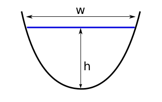
Parabolic shape with one degree of freedom, which makes it particulary useful for the bed inversion: if \(S\) and \(w\) are known:
The parabola is defined by the single bed-shape parameter \(P_s = 4 h / w^2\). Very small values of this parameter imply very flat shapes, unrealistically sensitive to changes in \(h\). For this reason, the default in OGGM is to use the mixed flowline model.
MixedFlowline
A combination of trapezoidal and parabolic flowlines. If the bed shape parameter \(P_s\) is below a certain threshold, a trapezoidal shape is used instead.
MUSCLSuperBeeModel
A shallow ice model with improved numerics ensuring mass-conservation in very steep walls [Jarosch_etal_2013]. The model is currently in development to account for various bed shapes and tributaries and will likely become the default in OGGM.
Glacier tributaries
Glaciers in OGGM have a main centerline and, sometimes, one or more tributaries (which can themsleves also have tributaries, see Centerlines). The number of these tributaries depends on many factors, but most of the time the algorithm works well.
The main flowline and its tributaries are all handled the same way and are modelled individually. The difference is that tributaries can transport mass to the branch they are flowing to. Numerically, this mass transport is handled by adding an element at the end of the flowline with the same properties (with, thickness...) as the last grid point, with the difference that the slope \(\alpha\) is computed with respect to the altitude of the point they are flowing to. The ice flux is then computed normally and transferred to the downlying branch.
The computation of the ice flux is always done first from the lowest order branches (without tributaries) to the highest ones, ensuring a correct mass-redistribution. The angle between tributary and main branch ensures that the former is not decoupled from the latter. If the angle is positive or if no ice is present at the end of the tributary, no mass exchange occurs.
References
| [Cuffey_Paterson_2010] | (1, 2) Cuffey, K., and W. S. B. Paterson (2010). The Physics of Glaciers, Butterworth‐Heinemann, Oxford, U.K. |
| [Farinotti_etal_2009] | Farinotti, D., Huss, M., Bauder, A., Funk, M., & Truffer, M. (2009). A method to estimate the ice volume and ice-thickness distribution of alpine glaciers. Journal of Glaciology, 55 (191), 422–430. |
| [Golledge_Levy_2011] | (1, 2) Golledge, N. R., and Levy, R. H. (2011). Geometry and dynamics of an East Antarctic Ice Sheet outlet glacier, under past and present climates. Journal of Geophysical Research: Earth Surface, 116(3), 1–13. |
| [Jarosch_etal_2013] | (1, 2) Jarosch, a. H., Schoof, C. G., & Anslow, F. S. (2013). Restoring mass conservation to shallow ice flow models over complex terrain. Cryosphere, 7(1), 229–240. http://doi.org/10.5194/tc-7-229-2013 |
| [Oerlemans_1997] | (1, 2) Oerlemans, J. (1997). A flowline model for Nigardsbreen, Norway: projection of future glacier length based on dynamic calibration with the historic record. Journal of Glaciology, 24, 382–389. |