Ice dynamics flowline model (default)#
The standard geometry evolution model in OGGM is a depth-integrated flowline model. The equations for the isothermal shallow ice are solved along the glacier centerline(s), computed to represent best the flow of ice along the glacier (see for example antarcticglaciers.org for a general introduction about the various types of glacier models).
Ice flow#
Let \(S\) be the area of a cross-section perpendicular to the flowline. It has a width \(w\) and a thickness \(h\) and, in this example, a parabolic bed shape.
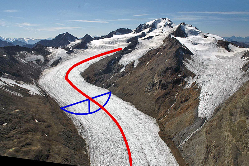
Example of a cross-section along the glacier flowline. Background image from http://www.swisseduc.ch/glaciers/alps/hintereisferner/index-de.html#
Volume conservation for this discrete element implies:
where \(\dot{m}\) is the mass balance, \(q = u S\) the flux of ice, and \(u\) the depth-integrated ice velocity ([Cuffey_Paterson_2010], p 310). This velocity can be computed from Glen’s flow law as a function of the basal shear stress \(\tau\):
where u_d and u_s are respectively the speed of ice coming from its deformation and sliding (n is equal to 3). Thus, the first term is for ice deformation and the second term is to account for basal sliding, see e.g. [Oerlemans_1997] or [Golledge_Levy_2011]. It introduces an additional free parameter \(f_s\) and will therefore be ignored in a first approach. The deformation parameter \(f_d\) is better constrained and relates to Glen’s temperature‐dependent creep parameter \(A\):
The basal shear stress \(\tau\) depends for example on the geometry of the bed [Cuffey_Paterson_2010]. Currently it is assumed to be equal to the driving stress \(\tau_d\):
where \(\alpha\) is the slope of the flowline, \(\rho\) the density
of ice and g the Earth gravity acceleration.
Both the FluxBasedModel and the MUSCLSuperBeeModel solve
for these equations, but with different numerical schemes.
Bed shapes#
OGGM implements a number of possible bed-shapes. Currently the shape has no direct influence on the shear stress (i.e. Cuffey and Paterson’s “shape factor” is not considered), but the shape will still have a considerable influence on glacier dynamics:
the width change as a result of mass transport will be different for each shape, thus influencing the mass balance term \(w \, \dot{m}\).
with all other things held constant, a change in the cross-section area \(\partial S / \partial t\) due to mass convergence/divergence will result in a different \(\partial h / \partial t\) and thus in different shear stress computation at the next time step.
Rectangular#
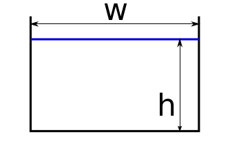
The simplest shape. The glacier width does not change with ice thickness.
Trapezoidal#
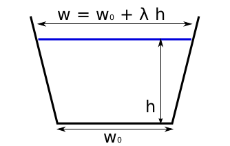
Trapezoidal shape with two degrees of freedom. The width change with thickness depends on \(\lambda\). The angle \(\beta\) of the side wall (as defined from the horizontal plane, i.e. \(\lambda = 0 \rightarrow \beta = 90^{\circ}\)) is defined by:
[Golledge_Levy_2011] uses \(\lambda = 2\) (a 45° wall angle) which is the default in OGGM as of version 1.4 (it used to be \(\lambda = 1\), a 63° wall angle).
Parabolic#
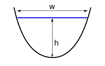
Parabolic shape with one degree of freedom, which makes it particularly useful for the bed inversion. If \(S\) and \(w\) are known:
The parabola is defined by the bed-shape parameter \(P_s = 4 h / w^2\) 1. Very small values of this parameter imply very flat shapes, unrealistically sensitive to changes in \(h\). For this reason, the default in OGGM is to use the mixed flowline model described below.
- 1
the local thickness \(y\) of the parabolic bed can be described by \(y = h − P_s x^2\). At \(x = w / 2\), \(y = 0\) and therefore \(P_s = 4 h / w^2\).
Mixed#
A combination of rectangular, trapezoidal and parabolic shapes.
Note
The default in OGGM is to used mixed flowlines, following these rules:
elevation-band flowlines have a trapezoid bed everywhere, except on the glacier forefront where the bed is parabolic (computed from the valley topography).
geometrical centerlines have a parabolic bed shape, with two exceptions:
if the glacier section touches an ice-divide or a neighboring tributary catchment outline, the bed is considered to be rectangular;
if the parabolic shape parameter \(P_s\) is below a certain threshold, a trapezoidal shape is used. Indeed, flat parabolas tend to be very sensitive to small changes in \(h\), which is undesired.
Numerics#
Semi-implicit model (new default in v1.6)#
This model solves a diffusion equation for the ice thickness \(h\), assuming a trapezoidal bed (Equation 10 in [Oerlemans_1997]). Numerically the equation is implemented using the present time-step diffusivity \(D\) but the future time-step surface slope \(\partial (b + h) / \partial x\) (with the glacier bed \(b\)), hence the name semi-implicit.
The solution of this equation involves a matrix inversion, which makes a single solving step around 1.5 times slower compared to the “Flux-based” model. However, the scheme is more stable hence each single solving step can use a three-time larger \(\Delta t\). Overall this halves the total runtime.
With the increased stability, we did not see numerical instabilities like for the “Flux-based” model (see Ice velocities in OGGM are sometimes noisy or unrealistic. How so?). But as the underlying equation is the same, we see the same non-mass-conserving behaviour in very steep slopes [Jarosch_etal_2013].
In summary, the Semi-implicit model is faster and more robust than the “Flux-based” model, but less flexible (currently only working with a single trapezoidal flowline).
“Flux-based” model#
Most flowline models treat the volume conservation equation as a diffusion problem, taking advantage of the robust numerical solutions available for this type of equations. The problem with this approach is that it implies developing the \(\partial S / \partial t\) term to solve for ice thickness \(h\) directly, thus implying different diffusion equations for different bed geometries (e.g. [Oerlemans_1997] with a trapezoidal bed).
The OGGM “flux based” model solves for the \(\nabla \cdot q\) term (hence the name). The strong advantage of this method is that the numerical equations are the same for any bed shape, considerably simplifying the implementation. Similar to the “diffusion approach”, the model is not mass-conserving in very steep slopes [Jarosch_etal_2013].
The numerical scheme implemented in OGGM is tested against Alex Jarosch’s MUSCLSuperBee Model (see below) and Hans Oerleman’s diffusion model for various idealized cases. For all cases but the steep slope, the model performs very well.
In order to increase the stability and speed of the computations, we solve the numerical equations on a forward staggered grid and we use an adaptive time stepping scheme.
See Ice velocities in OGGM are sometimes noisy or unrealistic. How so? for an ongoing discussion about the limitations of OGGM’s “Flux-based” scheme!
MUSCLSuperBeeModel#
A shallow ice model with improved numerics ensuring mass-conservation in very steep walls [Jarosch_etal_2013]. The model is currently used only as reference benchmark for the other models.
Glacier tributaries#
Glaciers in OGGM have a main centerline and, sometimes, one or more tributaries (which can themselves also have tributaries, see Glacier flowlines). The number of these tributaries depends on many factors, but most of the time the algorithm works well.
The main flowline and its tributaries are all modelled individually. At the end of a time step, the tributaries will transport mass to the branch they are flowing to. Numerically, this mass transport is handled by adding an element at the end of the flowline with the same properties (width, thickness …) as the last grid point, with the difference that the slope \(\alpha\) is computed with respect to the altitude of the point they are flowing to. The ice flux is then computed as usual and transferred to the downlying branch.
The computation of the ice flux is always done first from the lowest order branches (without tributaries) to the highest ones, ensuring a correct mass-redistribution. The use of the slope between the tributary and main branch ensures that the former is not dynamical coupled to the latter. If the angle is positive or if no ice is present at the end of the tributary, no mass exchange occurs.
References#
- Cuffey_Paterson_2010(1,2)
Cuffey, K., and W. S. B. Paterson (2010). The Physics of Glaciers, Butterworth‐Heinemann, Oxford, U.K.
- Golledge_Levy_2011(1,2)
Golledge, N. R., and Levy, R. H. (2011). Geometry and dynamics of an East Antarctic Ice Sheet outlet glacier, under past and present climates. Journal of Geophysical Research: Earth Surface, 116(3), 1–13.
- Jarosch_etal_2013(1,2,3)
Jarosch, a. H., Schoof, C. G., & Anslow, F. S. (2013). Restoring mass conservation to shallow ice flow models over complex terrain. Cryosphere, 7(1), 229–240. http://doi.org/10.5194/tc-7-229-2013
- Oerlemans_1997(1,2,3)
Oerlemans, J. (1997). A flowline model for Nigardsbreen, Norway: projection of future glacier length based on dynamic calibration with the historic record. Journal of Glaciology, 24, 382–389.